Loan Default Prediction in Retail Banking with MLOps

The subject

Personal loans are a major revenue source for retail banks, and their Achilles’ heel: every unanticipated default is written off. The dataset holds 10,000 customer records with 1,851 defaults (18.5%) and seven variables, including outstanding credit lines, total debt, income, tenure and FICO score. Two questions follow. What is each customer’s probability of default, and how does that model end up serving a credit decision rather than sitting in a notebook.

Reading the data before reaching for a model

One variable, the number of outstanding credit lines, decides most of the book on its own. Below two lines, no customer defaults. At five lines, 99.8% do. A single rule, default expected above four credit lines, misclassifies just 41 customers out of the 1,953 held out for testing, which is 97.9% accuracy with no model at all.

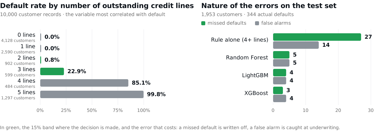
That baseline reframes the whole project. The 15% of customers holding two or three credit lines are where the decision is genuinely uncertain, and they carry 27 of the baseline’s 41 errors. Inside that band the separation comes from elsewhere: median FICO score of 590 for defaulters against 647 for the rest, debt-to-income ratio of 0.21 against 0.16, three years of tenure against five. That is the signal the engineered features have to capture, and the reason a headline accuracy figure is not, by itself, an argument.

The pipeline

• Cleaning: an IQR factor tuned per variable (2.80 on outstanding loan amount, 3.90 on total debt, 1.90 on income, 2.00 on FICO score), combined with a 3 sigma z-score filter. 237 records removed, 2.4% of the dataset.
• Feature engineering: debt-to-income ratio, credit-to-income ratio, gap to a 700 FICO reference and normalized FICO score, added to the raw variables.
• Split: 60/20/20, so 5,857 training, 1,953 validation and 1,953 test records. SMOTE oversampling followed by random undersampling is applied to the training set only, leaving validation and test at their natural default rate so that measured performance stays representative of the real book.

Those IQR factors are the step worth defending. Applied at the textbook 1.5, the same filter drops 840 records and takes 658 defaults with them, a third of the minority class gone before training starts.

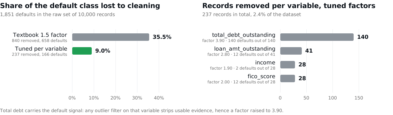
The reason is structural. High total debt is not noise here, it is the default signal, so any threshold on that variable cuts into the very population the model has to catch. Raising its factor to 3.90 brings the loss down to 9% of defaults, and even then the 140 records it still removes are defaults, every one of them. An outlier rule read as a hygiene step would have silently biased the training set.

Tuning and traceability

Optuna searches each model family against a single objective, a composite score weighting 0.4 AUC-ROC, 0.3 Precision-Recall AUC, 0.2 F1, 0.05 recall and 0.05 precision. Writing the trade-off as one number pushes the search toward ranking quality first and threshold behavior second, instead of letting accuracy reward a model that plays the majority class.

288 runs across four MLflow experiments (logistic regression, random forest, XGBoost, LightGBM) log their parameters, metrics, confusion matrix, model signature and a versioned model tag, each tied to the commit that produced it. Any result on this page can be traced back to the run that produced it.

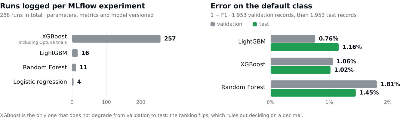
The ledger also settles the model choice. LightGBM leads in validation and loses on test, XGBoost is the only family that does not degrade between the two. Picking on the validation decimal alone would have shipped the wrong model.

Results

On the 1,953-record test set, with 344 actual defaults:

• XGBoost: 99.64% accuracy, 7 errors (4 false positives, 3 missed defaults), 99.1% recall on the default class.
• LightGBM: 99.59%, 8 errors.
• Random Forest: 99.49%, 10 errors.
• Logistic regression, kept as the readable reference: 98.3% accuracy and 0.949 F1 in validation, with an AUC-ROC of 0.999 that says more about the data than about the model.

Read against the baseline, the tuned model removes 34 of its 41 errors, and the gain lands where it costs: 27 defaults slip through the rule against 3 through XGBoost. False alarms fall from 14 to 4, but they were the cheap error to start with, since underwriting catches them before any money leaves. That asymmetry, not the third decimal of an accuracy score, is what a risk team needs to see.

From model to product

The Streamlit application is the console for the whole lifecycle rather than a prediction demo: exploratory analysis, feature engineering, launching a tracked run with a chosen model, feature subset and trial budget, browsing the MLflow artifact registry, and scoring a customer against the production model.

Packaging follows: Poetry-locked dependencies, a Python 3.12 slim image with a Streamlit health check, and a GitHub Actions pipeline that formats, lints and health-checks the container on every pull request before pushing a date-tagged image to Docker Hub and to Amazon ECR for deployment on ECS in eu-west-3.

What the project demonstrates

Evaluation discipline ahead of algorithmic sophistication: a baseline that qualifies the real difficulty before any model is trained, a success metric written as a business trade-off rather than an accuracy figure, and a run history that makes each choice defensible after the fact. Those reflexes transfer directly to LLM systems, where the reference point, the scoring rule and the traceability of every run matter more than the model on top.